Part A - Image Warping and Mosaicing

Part 1: Shoot the Pictures

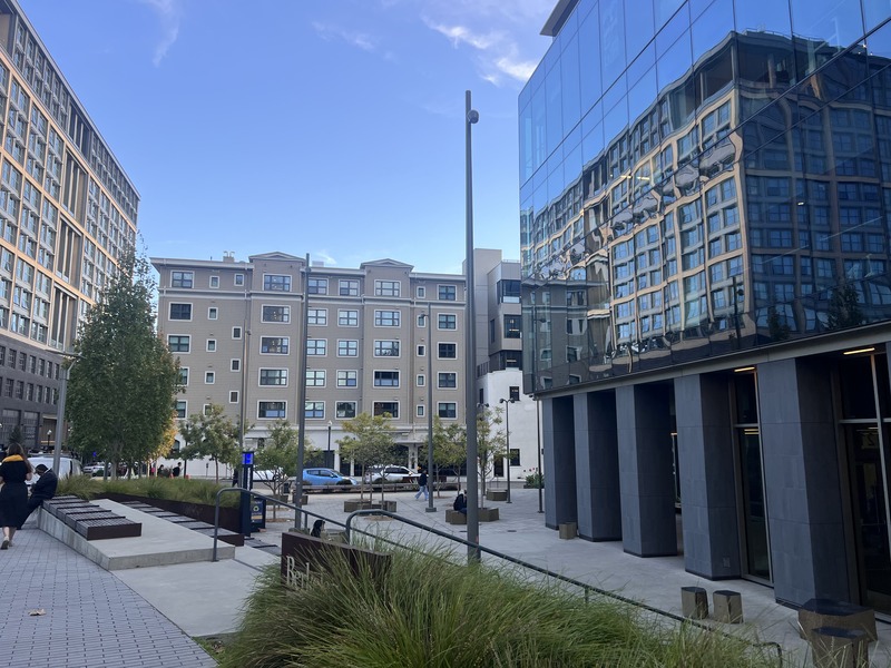
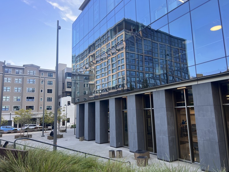
I took photos with my phone from three distinct locations, rotating the camera at each spot.

Original images:

Part 2: Recover Homography Matrices

Homography Equation

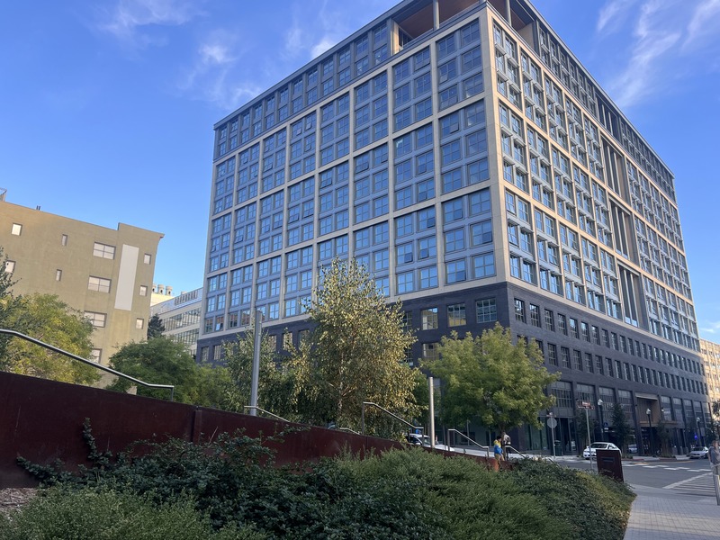
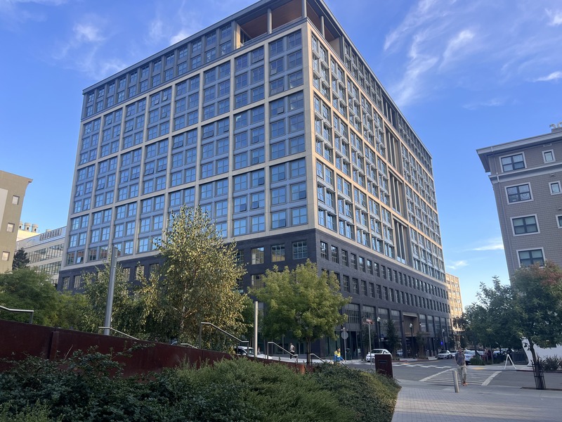
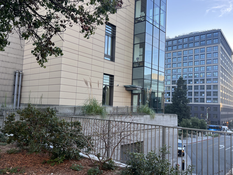
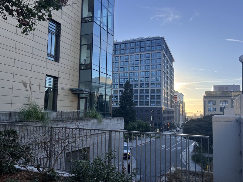
A homography matrix \( H \) relates points in one image to corresponding points in another image:

Expanding above,

Linear System Setup

For each pair of corresponding points \( (x, y) \) and \( (x', y') \), two equations can be set up:

Matrix Formulation

We build a matrix \( A \) from the equations above. For each point pair, we have:

This produces a system \( A \cdot h = 0 \), where \( h \) is a vector of the 8 unknowns in \( H \).

Solving Using SVD

To solve for \( H \), I used Singular Value Decomposition (SVD) to estimate Homography Matrix.

Part 3: Image Warping

The warpImage function takes an image and a homography matrix H as inputs to warp the image according to the transformation described by H. The function defines the four corners of the image and applies the inverse of the homography matrix to transform these corners, calculating the minimum and maximum x and y coordinates to determine the size of the output canvas. If the transformed coordinates extend beyond the image boundaries, it calculates offsets to ensure the entire transformed image fits within the new canvas dimensions.

The function uses these transformed coordinates to generate a polygon that encompasses the new boundaries. It then constructs the homogeneous coordinates of points within this polygon and maps them back to the source image using the homography matrix. To perform this transformation, the function uses inverse mapping and normalizes the coordinates.

Next, it creates a grid of points corresponding to the pixel locations in the source image, and initializes an empty canvas for the warped image with the computed size. The function then applies scipy.interpolate.griddata to interpolate pixel values from the source image for each channel individually. It uses the nearest neighbor method to fill the pixels in the warped image based on the transformed coordinates.

Finally, the function assigns the interpolated pixel values to the appropriate locations in the new canvas.

Here are the wraped results:

Part 4: Rectification

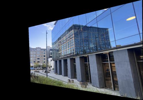
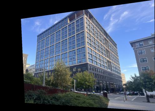
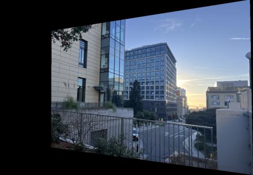
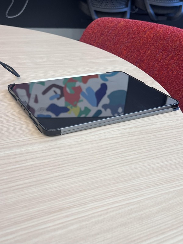
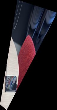
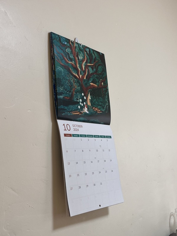
To rectify images, the warpImage function is used with inverse warping. Inverse warping involves applying the inverse of the homography matrix, which transforms the coordinates of the distorted image back to their original, undistorted positions.

By using inverse warping, the function interpolates pixel values from the source image to fit a new, rectified view. The result is an image that appears as if it were taken from a frontal perspective.

Part 5: Blend the images into a mosaic

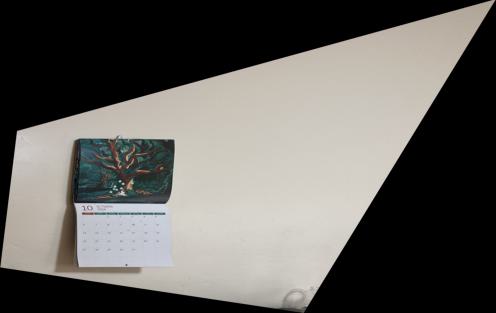
This process combines two images using Laplacian stack from project 2. The blending process involves the following steps:

1. Image Warping: The second image is warped using warpImage function from previous parts.
2. Canvas Creation: A larger canvas is created to accommodate both the first and the warped second image.
3. Mask Generation: A mask is generated to differentiate between regions where only the first image, only the second image, and the overlapping areas exist. In the overlapping regions, a gradient is created using distance transforms, which allows for a smooth transition between the two images.
4. Gaussian and Laplacian Pyramids: Gaussian and Laplacian pyramids are created for both images. The mask is also processed with Gaussian pyramids to match the levels of the image pyramids.
5. Blending Process: The images are blended using the pyramids and the generated mask. The mask ensures a smooth transition in the overlapping region, where the blending weights vary gradually from one image to the other based on the gradient values.

Here are final results:

Reflection

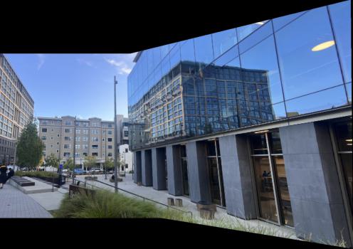
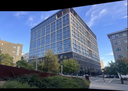
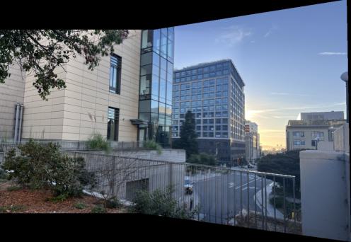
Working with front warping and inverse warping was tricky and required careful consideration of coordinate transformations. It took a significant amount of time to debug, but it was interesting overall as I could experiment with distorting images from different perspectives.

Part B - Feature Matching for Autostitching

Part 1: Harris Interest Point Detector

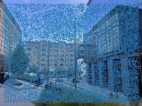
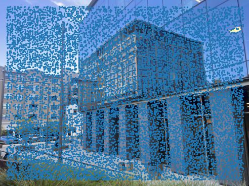
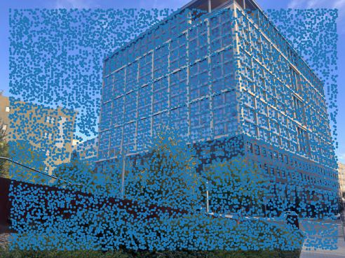
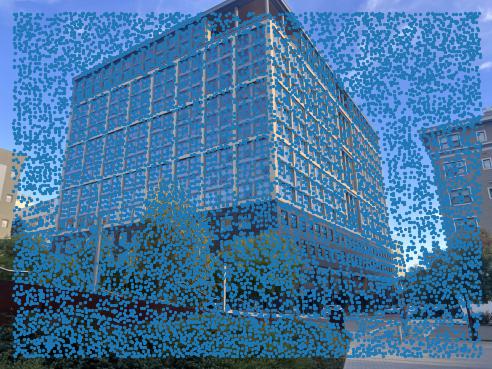
The Harris Corner Detector identifies corners by finding points in an image where the intensity changes significantly in both the x and y directions.

Process Overview:

1. Compute Gradients: Calculate the intensity changes (gradients) in the x and y directions.
2. Corner Response: Use these gradients to compute a corner response score, which highlights likely corner points.
3. Thresholding: Keep only points with high corner scores.

I used the provided harris.py code to apply this process. Below is a figure showing the Harris corners overlaid on the image.

Part 2: Adaptive Non-Maximal Suppression

Approach:

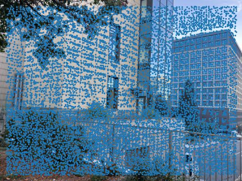
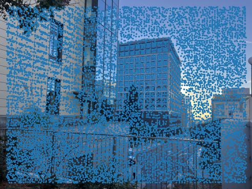
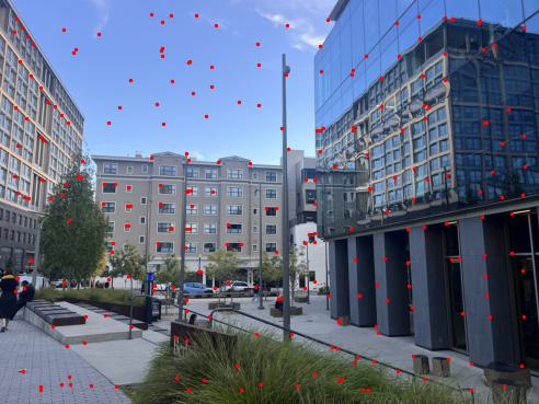
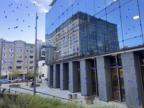
1. Compute Corner Responses: For each point, retrieve the Harris corner response (strength) from h based on the input coordinates coords.
2. Sort by Response Strength: Sort the coordinates in descending order of their corner response values.
3. Calculate Radius for Suppression: For each point, calculate a radius representing the minimum distance to any higher-ranked point. This radius is constrained by c_robust=0.9, ensuring that only points with significantly lower responses are suppressed.
4. Select Top Features: Choose the points with the largest radii up to the specified maximum number of features max_features=250. These points represent the most robust features with good spatial distribution.

The anms function effectively filters out non-robust features while keeping the well-distributed corners.
The results below show the key points selected through ANMS:

Part 3: Feature Descriptor extraction

Approach:

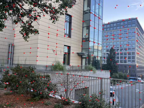
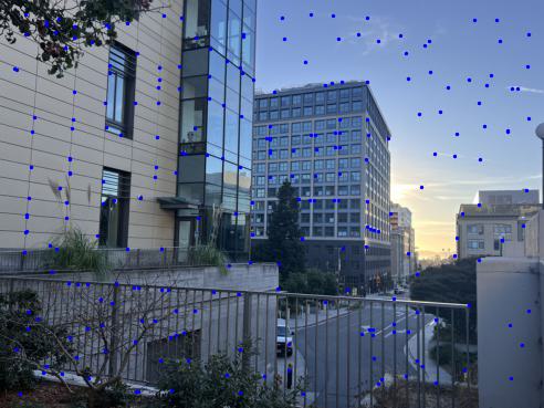
1. Patch Extraction: For each interest point, a 40x40 patch centered on the point is extracted from the image.
2. Downsampling to 8x8: The patch is downsampled to an 8x8 patch.
3. Normalization: The extracted patch is bias/gain-normalized by subtracting the mean and dividing by the standard deviation.

The resulting feature descriptors are used to match the set of images.

Below are the extracted and normalized patches of one of the images:

Part 4: Feature Matching

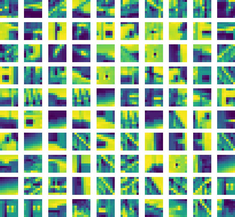
The feature matching process compares descriptors from two images to identify corresponding features.

Approach:

1. Flatten Descriptors: The descriptors from both images are flattened for easier distance calculation, transforming each descriptor into a 1D vector.
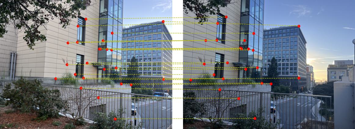
2. Distance Calculation: For each descriptor in descriptor1 (from Image 1), the Euclidean distance to every descriptor in descriptor2 (from Image 2) is computed.
3. Find Closest Matches: The two descriptors with the smallest distances are identified. The nearest descriptor (closest match) and the second nearest are used for comparison.
4. Lowe's Ratio Test: If the distance to the nearest match is smaller (within the ratio_threshold) than the distance to the second nearest match, the match is retained.
5. Store Matches: The matched key points are stored.

This matching process yields pairs of points from both images that are likely to correspond.
Here are the results of the matched features across the set of images:

Part 5: RANSAC

Approach:

1. Random Sampling of Feature Pairs: In each iteration, four feature pairs are randomly selected from the points in both images.
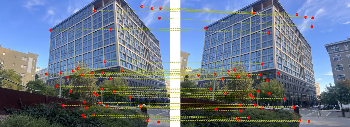
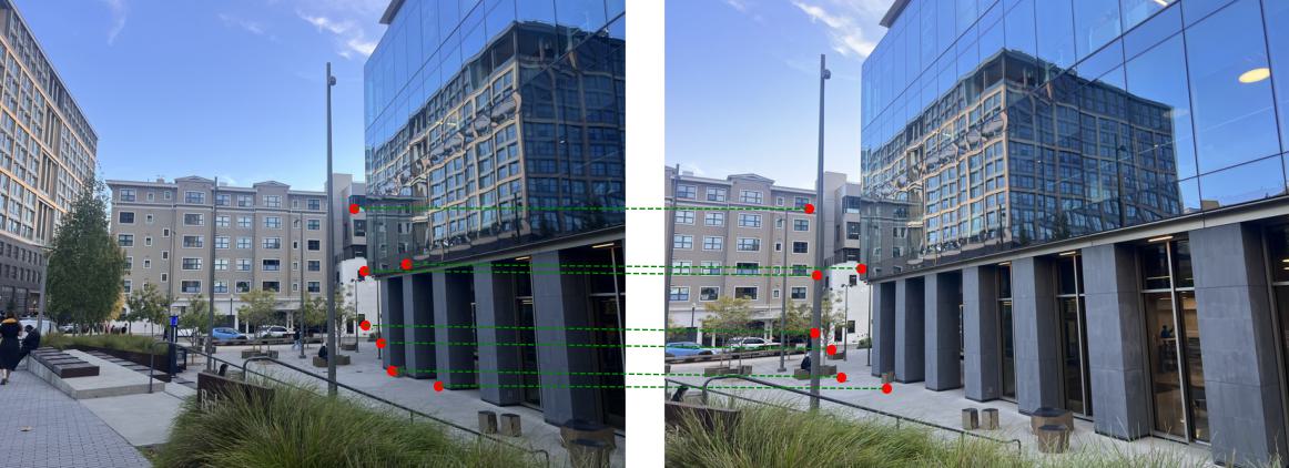
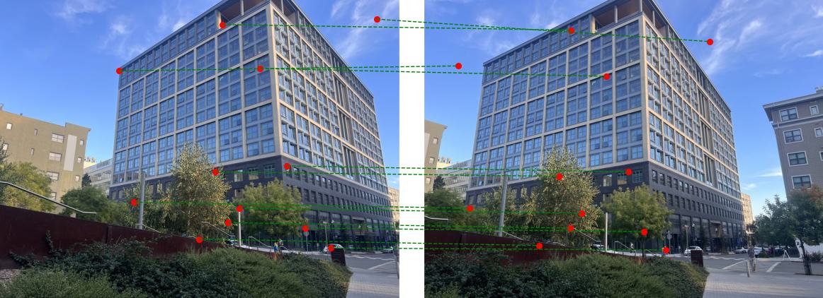
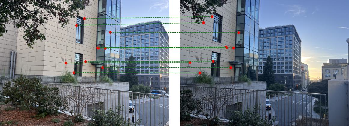
2. Compute Homography Matrix: A homography matrix H is computed using the selected pairs.
3. Calculate Inliers: Using H, points from the first image are transformed, and their distances to corresponding points in the second image are calculated. If the distance is below a threshold, the point pair is considered an inlier.
4. Identify Best Inliers: The set of inliers is tracked across all iterations, and the H with the largest inlier set is retained as the best fit.
5. Recompute Final Homography: After finding the best set of inliers, a final H is computed using all inliers to increase accuracy.

By iteratively refining the homography based on inliers, RANSAC provides a robust estimate of the transformation.
Below are the results of the RANSAC process across the set of images:

Mosaics

Below are the results of three mosaics: automatically stitched and manually stitched, respectively.

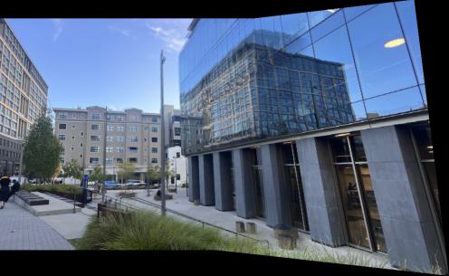
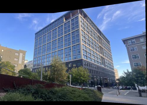
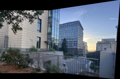
There is not a significant visual difference between the manually stitched and automatically stitched versions. Both methods align the images well. The automatic stitching algorithm effectively aligns key features without noticeable misalignments.